Adversarially Constrained Alphabet Channel Capacity
In information theory literature, a common setup is that of the imperfect channel. Typically, two people are trying to communicate with one another across a channel. The sender can send one symbol out of a given alphabet at each step, and after they send their symbol an "adversary" possibly introduces error by modifying their symbol with some probability before it gets received by the receiver. This is a reasonable model for many communication channels that exist in the real world, as we often encounter loss in our communication channels in the form of random bit flips.
I became interested in a related problem, which is a setup where the "adversary" acts before the sender does, instead of after. Concretely, at each step the "adversary" somehow constrains the possibilities that are open to the sender. In this blog post I will talk specifically about the scenario where the alphabet of possible symbols to be sent over the channel has size \(m\), and at each step the adversary chooses \(n < m\) of those as the options for the sender to choose from.
The simplest nontrivial case is when \(m=3\) and \(n=2\). Let us define our alphabet as \(\{0,1,2\}\). At every step, our adversary will choose two out of these three options, and our sender will need to select one of the two to send to the receiver. We assume there is no error or loss in the communication channel after a symbol is selected and sent.
We want to know how many bits of information we can actually convey at each step, and what strategy we can use to maximize the information conveyed. There are actually several slightly different formulations of this problem, which drastically change the solution. Let us examine a few.
Active Adversary, Deterministic Encoding Scheme
For this case, we assume that the encoding/decoding scheme we use is deterministic, and that the adversary might have knowledge of it and can therefore choose which options to give us to minimize the information we can send.
One way to think about this is to suppose we are trying to eventually convey one specific possibility out of set \(X\) of length \(x\) total possible messages. For example if we were trying to send a 4-bit binary message, we would be trying to convey one out of the 16 possible 4-bit binary strings. At each step, we can think about how many remaining options we are able to "eliminate". Let \(X_p\subset X\) be the remaining options conditional on receiving \(p\) for \(p\in\{0,1,2\}\). Clearly we need that \(X_p\cup X_q = X\) for \(p\neq q\).
It is not hard to prove that in this formulation, the optimal arrangement is to let \(\vert X_p\vert = \frac23\) for all \(p\). We can therefore eliminate \(\lfloor\frac13\rfloor\) of the options at each step. This suggests a channel capacity of \(\log_2\frac32\approx 0.585\) bits per step.
However, we have a problem. Using this approach, we cannot distinguish between the last two possible messages. In fact, we can prove that there is no encoding that allows us to do this.
Proof. Suppose we are just trying to convey a single bit of information (let's call the options High and Low). Suppose for contradiction that there exists a minimal number of steps \(s\) that is required to convey this bit of information. This means that after \(s-1\) steps, there must be at least one adversarial strategy that results in the sender sending a sequence of symbols that cannot be definitively interpreted as either High nor Low. Then in the following step, by simple pigeonhole argument, there must either be only one out of the three possible symbols that, when received, would definitively convey to the receiver either High or Low. But then the adversary could simply prevent us from sending that symbol, which would prevent us from conveying either High or Low. That means we cannot definitively convey at least one of High or Low after \(s\) steps, which is a contradiction.
This proof was so surprising to me when I discovered it that I actually formalized it in Rocq to make sure I wasn't making a logical error. But it's true, we can't guarantee that we can convey a single bit! This feels extremely surprising to me because it means we can narrow down our space of possibilities exponentially quickly from any arbitrary number, all the way down to 2, but we can't necessarily differentiate between the last two options!
What's more, let's say we have two separate messages we want to send. We can definitely narrow down message 1 to two options (\(a\) and \(b\)), and we can definitely narrow down message 2 to two options (\(c\) and \(d\)). Then, it looks like we are stuck, but actually we can craft a new metamessage with 4 options:
- "message 1 has value a, message 2 has value c"
- "message 1 has value a, message 2 has value d"
- "message 1 has value b, message 2 has value c"
- "message 1 has value b, message 2 has value d"
Going back to the general case where we have an alphabet of size \(m\), out of which ad adversary picks \(n\) options that are valid for us to send, we can show:
- for any \(n\leq\lceil\frac m2\rceil\), we have this problem where we cannot distinguish between multiple messages at the end, and
- for all larger \(n\) we are definitely able to distinguish between messages in a finite number of steps.
Active Adversary, Nondeterministic Encoding Scheme
Assuming a shared source of randomness between the sender and the receiver, we can use the same approach as before, except that at each step we randomly choose from \(\{0,1,2\}\) with equal probability and add that value to the message (modulo 3). This ensures that the adversary cannot choose a strategy that prevents us from disambiguating between the last 2 options, and the probability that we are able to convey our message definitively approaches 1 as the number of steps approaches infinity.
We might expect that the best solution is again to set \(\vert X_s\vert = \frac23\) for all \(s\), which as we calculated yields a channel capacity of \(\log_2\frac32\approx 0.585\) bits per step. However, let's see if we can do better.
We introduce new notation. We consider just one step of our encoding/decoding. Let our encoding alphabet be \(A\), which in this specific case is \(A=\{0,1,2\}\). Let \(M\) be the set of messages we are trying to disambiguate between at this time step. Our encoding scheme should be such that after this step, we are left with a set \(M_a \subseteq M\) of possible options, which depends on the specific value \(a\in A\) that we choose to send. We define \(p_a=\frac{\vert M_a \vert}{\vert M \vert}\).
For a given encoding scheme and each subset \(S\subseteq A\), let \(M_S\) be the set of messages \(m\in M\) such that \(x\in M_a\) for all \(a\in S\) and \(x\notin M_b\) for all \(b\notin M_b\). Then, let \(p_S = \frac{\vert M_S\vert }{\vert M\vert }\).
As an example, suppose we had 3 possible messages in the space of valid messages: \(x\), \(y\), or \(z\). Suppose also that our encoding system states that if we receive a \(0\) we can safely conclude that the actual message must be either \(y\) or \(z\), but not \(x\). Similarly, \(1\) conveys \(x\) or \(z\) and \(2\) conveys \(x\) or \(y\). Then \(M_\emptyset = M_{\{0\}} = M_{\{1\}} = M_{\{2\}} = M_{\{0, 1, 2\}} = \emptyset\), while \(M_{\{0, 1\}}=\{z\}\) and \(M_{\{0, 2\}}=\{y\}\) and \(M_{\{1, 2\}}=\{x\}\). This means \(p_{\{0,1\}}=p_{\{0,2\}}=p_{\{1,2\}}=\frac13\).
As a side note, \(p_{\{a\}}\) is not necessarily equal to \(p_a\) (as defined in the previous paragraphs). In fact, these are rarely equal. Almost always, \(p_{\{a\}}\lt p_a\).
Let's observe some properties of \(p_S\).
First, it is obvious that the values of \(p_S\) must sum to 1. More mathematically, \[\sum_{S\subseteq A}p_S = 1\]
Second, for any valid encoding scheme for a variation where the opponent gives you \(n\) choices out of \(m\) total characters in the alphabet, then \(p_S = 0\) for all \(S\) such that \(\vert S \vert \leq m - n\). If this were nonzero, then suppose we were trying to encode some message from \(M_S\). If the opponent gave us some subset of \(A\setminus S\), then we would have no valid options to send to encode our message.
Any encoding that obeys these two properties is a valid encoding. However, we can make a few more observations about optimal encodings (encodings with the highest expected amount of information conveyed).
In an optimal encoding, when given a choice between multiple valid choices for which symbol to send, we should always choose the one that cuts down the message space as much as possible. More precisely, if we are trying to convey a message in \(M_S\), and we are allowed the choices \(T\subset A\) to send, then we should choose to send \[\text{arg}\min_{x'\in S \cap T}p_{x'}\]
Consequently, since the adversary can only remove \(m-n\) options, this means that we will never need to send the symbol \(s\) with the \((m-n+2)\)th or larger \(p_s\), which means \(M_S\) does not need to be in \(M_s\). Therefore, we can conclude that \(p_S=0\) for all \(S\) such that \(\vert S \vert \neq m - n + 1\).
We can now use these values \(p_S\) to quantify how much information we can encode on average for a given encoding: \[\sum_{S\subseteq A : \vert S \vert = m - n + 1}\left(\sum_{T\subseteq A : \vert T \vert = n} -\frac{p_S}{\binom{m}{n}}\log_2\left(\min_{x\in S \cap T}p_x\right)\right)\]
This can be simplified a bit, but it does require some nonstandard notation. We define \(\min\limits_{S}{}^{(n)}(f(S))\) to be the \(n\)th smallest value of \(f(s)\) over \(s\in S\). \[-\frac{1}{\binom{m}{n}}\sum_{S\subseteq A : \vert S \vert = m - n + 1}\left(p_S\sum_{i=1}^{m-n+1}\binom{m-i}{n-1}\log_2\left(\min_{x\in S}\!{}^{(i)}p_x\right)\right)\]
Unfortunately, this does not seem to be easily solvable in the general sense for arbitrary \(m\) and \(n\). But we can use it to solve for our \(m=3\), \(n=2\) case from before. We note that in this case, \(p_{\{0, 1\}}, p_{\{0, 2\}}, p_{\{1, 2\}}\) are symmetric such that we can assume without loss of generality that \(p_{\{0, 1\}} \leq p_{\{0, 2\}} \leq p_{\{1, 2\}}\).
Our expression for the expected information becomes: \[-\frac{1}{\binom{3}{2}}\sum_{S\subseteq A : \vert S \vert = 2}p_S\left(\binom{2}{1}\log_2\min_{x\in S}p_x + \binom{1}{1}\log_2\max_{x\in S}p_x\right)\] \[-\frac{1}{3}\left(p_{\{0,1\}}\left(2\log_2p_0 + \log_2p_1\right) + p_{\{0,2\}}\left(2\log_2p_0 + \log_2p_2\right) + p_{\{1,2\}}\left(2\log_2p_1 + \log_2p_2\right) \right)\] \[-\frac{1}{3}\left( (2 - 2p_{\{1, 2\}})\log_2(1-p_{\{1,2\}}) + (p_{\{0,1\}} + 2p_{\{1, 2\}})\log_2(1-p_{\{0,2\}}) + (1-p_{\{0,1\}})\log_2(1-p_{\{0,1\}}) \right)\]
This is still not super nice to work with, but we can find the partial derivatives, check boundary conditions, and find that the optimal values to maximize this expression are \(p_{\{0,1\}}=0\), \(p_{\{0,2\}}=p_{\{1,2\}}=\frac12\), for an expected information transfer rate of \(\frac23\) bits per step!
As a side note, this corresponds to setting \(2\) to convey nothing, and \(0\) and \(1\) to each convey one bit. In \(\frac23\) of cases, the adversary does not remove from us the possibility of sending whichever of \(0\) or \(1\) that we want to send, so we are able to convey a full bit of information, and in the last \(\frac13\) of cases, we are forced to send a dud \(2\).
Other Values of \(m\) and \(n\)
For larger values of \(m\) and \(n\), the values of \(p\) are not sufficiently symmetric to allow for the type of reasonably easy analysis that we did for the \((3,2)\) case. Solving them exactly would probably involve lots of casework. I have written a simulation for this maximization problem, though, and have some reasonable lower bounds for the bitrate values for some more cases. Here, I provide a chart of values I've found through simulation. Most are not proven to be optimal.
| 2 | 3 | 4 | 5 | 6 | 7 | 8 | 9 | |
|---|---|---|---|---|---|---|---|---|
| 2 | 1 (2) |
\(\frac23\) (2,1) |
0.5063797... | 0.4169017... | 0.3547072... | 0.3088933... | 0.2743758... | 0.2470715... |
| 3 | - | \(\log_23\) (3) |
\(\frac34\log_23\) (3,1) |
0.9561512... | 0.8272793... | 0.7302215... | 0.6531272... | 0.5927882... |
| 4 | - | - | 2 (4) |
\(\frac85\) (4,1) |
1.3348749... | 1.1932627... | 1.0782870... | \(\frac49\log_23+\frac5{18}\) (3,2,1,1,1,1) |
| 5 | - | - | - | \(\log_25\) (5) |
\(\frac56\log_25\) (5,1) |
\(\frac53\) (4,2,1) |
\(\frac{85}{56}\) (4,2,1,1) |
\(\frac{25}{18}\) (4,2,1,1,1) |
| 6 | - | - | - | - | \(\log_26\) (6) |
\(\frac67\log_26\) (6,1) |
\(\frac34\log_25+\frac3{14}\) (5,2,1) |
\(\frac23\log_25+\frac14\) (5,2,1,1) |
| 7 | - | - | - | - | - | \(\log_27\) (7) |
\(\frac78\log_27\) (7,1) |
\(\frac79\log_26+\frac7{36}\) (6,2,1) |
| 8 | - | - | - | - | - | - | 3 (8) |
\(\frac83\) (8,1) |
| 9 | - | - | - | - | - | - | - | \(\log_29\) (9) |
Nice and Ugly Solutions
You'll notice that some of these are just decimal approximations, while others are exact expressions. This is quite interesting: for some values, the simulation best solution is nice and orderly (more on that in a bit), while for others the best solution is kind of random-looking. It's not that I got a big decimal for all of them and only figured out the exact expression that results in that decimal. It's that the type of optimal solution is fundamentally different.
Nice Solutions
Let's examine the orderly solution type first. You'll notice that they underneath the expressions, I've included something like (4,2,1,1). For each number \(n\) in that tuple, it indicates that the solution contains \(n\) values in the alphabet that each map to a disjoint subset of size \(\frac1n\) of the total message space.
As an example, for this (4,2,1,1) solution to \(m=8\) and \(n=5\), this means the solution I found divides the message space into 4 quarters, \(q_1,q_2,q_3,q_4\). If we receive symbol \(a_1\), that corresponds to saying that the message we want to send is in \(q_1\), and similarly for \(a_2,a_3,a_4\). That's what the 4 represents in (4,2,1,1). The two means that \(a_5\) corresponds to saying the message is in \(q_1\) or \(q_2\), while \(a_6\) says the message is in \(q_3\) or \(q_4\). And finally, the two 1s means \(a_7\) and \(a_8\) don't convey any information at all.
I will refer to these types of solutions as nice solutions.
Ugly Solutions
What about the inexact solution values? Well, the simulation found a solution that's better than any of the possible nice solutions, but this better solution seems to be kind of random-looking (in a loose sense of the word "random"). For example, the best nice solution to the \(m=6\) and \(n=4\) case would be (in the tuple notation from above): (4,1,1). This yields an expected \(\frac43\) bits per step (which I'll refer to as a solution's score from now on). As nice as that is, that's not as good as the solution the simulation found, which is the following:
\(p_{\{0,1,2\}}=0.28974989498008397\)
\(p_{\{0,2,3\}}=0.1309123611045367\)
\(p_{\{0,2,4\}}=0.2684874741724991\)
\(p_{\{0,3,4\}}=0.021055956739389113\)
\(p_{\{0,3,5\}}=0.28979431300349134\)
(and \(p_S=0\) for all other \(S\)).
This random-looking solution yields a slightly improved score of 1.3348749.
From here on out I'll refer to these solutions with random-looking values as ugly solutions.
The Missing Middle
Notably absent from any of the cases I've explored is any kind of middle-ground solution. By this, I mean a solution that does not exactly conform to the way nice solutions are defined, but still has some nonzero rational values of \(p_S\) for some \(S\). This is not to say that such a solution can definitely never be optimal, but it sure looks like that might be the case.
More on Ugly Solutions
It is not clear to me why ugly solutions trump nice solutions for some values of \(m\) and \(n\) but not for others. My initial hypthesis is that for small enough values of \(m\) and \(n\), the fact that nice solutions are in a sense "quantized" means that there might be a big gap between, for example, the solutions (4,1,1) and (3,2,1), and these ugly solutions are kind of "halfway between" those two nice solutions.
It is clear there is some kind of "cost" to these random looking solutions versus the nice ones. For the (m,n)=(6,4) example, we can think about nice solutions of the form (x,5-x,1). As it turns out, the best value of x here is 4, which yields a score of \(\frac43\), as mentioned previously. A value of \(x=3\) yields a slightly lower score of 1.323308. It's not hard to show that the score can be calculated as \(\frac{2}{3}\log_{2}x+\frac{4}{15}\log_{2}(5-x)\). But if we were able to entirely unshackle ourselves from the realm of integers, the maximum for this function would be at \(x=3.57143\), resulting in a score of 1.36155. It's pretty clear we're getting nowhere near that value in practice with the random solutions.
We can in fact prove that ugly solutions always win for \(n=2\), and it seems they tend to win for other small values of \(n\) often as well. For example, more simulations showed that for \(m=13\) and \(n=5\), an ugly solution got a score of at least 1.043163677, while the best nice solution is (3,2,2,1,1,1,1,1,1) with a pitiful score of 1.02918138.
Classes of Nice Solutions
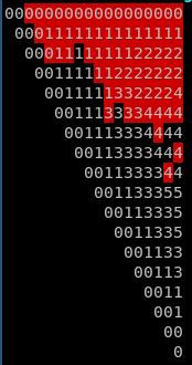
We can examine in more detail the concept of ugly solutions potentially appearing near boundaries between "classes" of nice solutions. We can somewhat arbitrarily define the "class" of a nice solution by taking its representational tuple, removing its first (largest) element, and also removing the trailing ones. So (3,2,2,1,1,1) is in the class (2,2), as are (2,2,2) and (5,2,2,1). (8) and (8,1) are both in the () class.
Now, we can plot the best nice solution by which class they belong to. In the image below, the columns represent values of \(m\) starting at 2, while the rows represent values of \(n\) starting at 2. Each digit represents a different optimal nice solution, though the digit itself has no direct relationship to the class that it represents.
Shaded locations mark cases where an ugly solution has been shown to best the optimal nice solution.